


This section presents an overview of the LIFE architecture and a description of the evaluation design (see Figs. 1, 2).

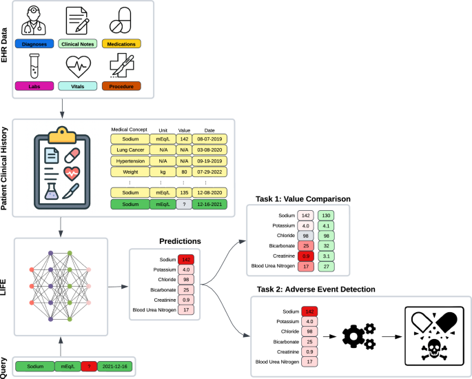
EHR observations and a query comprising a laboratory test, a unit of measure, and a date are input into LIFE to impute the corresponding laboratory value for that specific time point. We assessed these imputations within two scenarios. For the initial experiment (Task 1), we masked laboratory data from a patient’s clinical history, replaced the absent value through imputation, and then compared it with the actual measurement. In the subsequent experiment (Task 2), we employed LIFE’s laboratory value imputations as features within a downstream task focused on detecting adverse events.

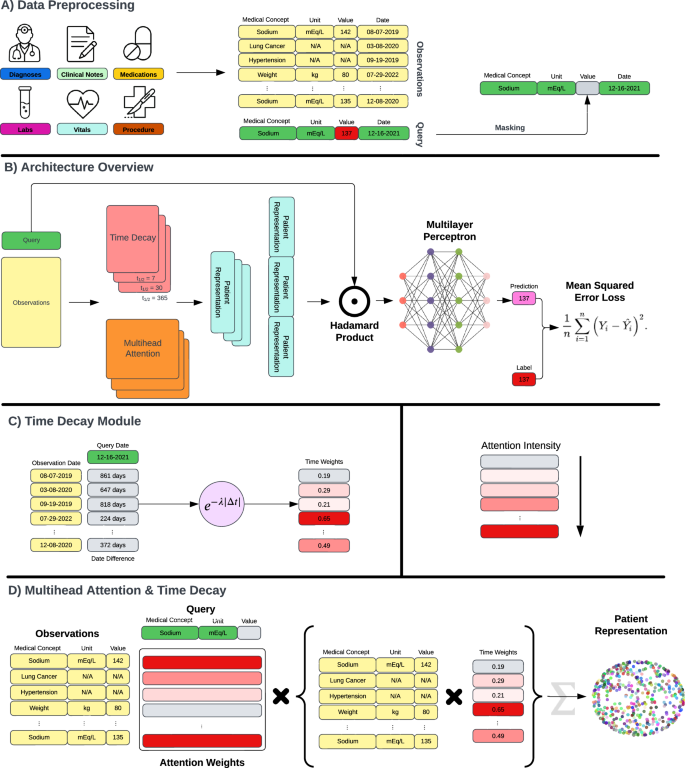
A The model’s inputs consist of a query, which includes a laboratory test, a unit of measure, and a date, along with EHR observations extracted from patient clinical records. During the training phase, each query is chosen randomly from the available patient laboratory data, and its value is masked before being fed into the model. B LIFE is constructed with time decay and multi-head attention layers, both contributing to the creation of patient embeddings. The multiple time decay modules compute observations across various time scales. The patient embeddings resulting from this process are then subjected to multiplication by the query using the Hadamard product. The concatenated result is passed through a multi-layer perceptron to generate a final prediction. Throughout the training iterations, the model predicts the masked values and aims to minimize the discrepancy between original and imputed values through Mean Square Loss. C The time decay module assigns weights to observations based on their proximity to the time point specified in the query. These weights are determined by calculating the time difference in days between each observation and the query and then applying an exponential decay function. D The multi-head attention module assigns weights to observations according to their medical significance relative to the query. This module takes three inputs: the query, the observations, and the weights computed by the time decay mechanism.
Dataset
We used de-identified EHRs from the Tempus Database (Tempus AI, Inc., Chicago, IL) for both model training and testing. This database contains de-identified, structured EHRs of oncology patients gathered from over 350 direct data connections across approximately 2000 healthcare institutions in the United States that order Tempus products and services. This study and the data used received IRB exempt determinations (Advarra Pro00042950 and Pro00072742) as it was deemed to not be human subjects research. Informed consent from people whose data was included and analysed was not required, as all data were de-identified prior to analysis in accordance with the IRB exemptions. We included in the study only patients with at least one continuous laboratory value in their clinical history. This led to a dataset of about 1.1 million patients, spanning the years 2000 to 2023, comprising about 65% females and 45% males, with a mean age of 69.1 years (standard deviation = 15.8) as of 2023.
For each patient, we aggregated general demographic details (i.e., age, sex, and race) and clinical descriptors. We included ICD-10 diagnosis codes, medications normalized to RxNorm, Current Procedural Terminology version 4 procedure codes, and vital signs and laboratory data normalized to LOINC. The vocabulary was composed of 29,454 medical concepts, leading to a dataset with an average of 727 records per patient.
The dataset contained 707 million laboratory values and 4788 distinct laboratory tests. In order to obtain meaningful predictions and not bias training because of data scarcity, we considered only the tests with at least 10,000 occurrences. This led to 344 distinct laboratory tests that were used as imputation targets in the evaluation.
The data was randomly split at the patient level into an 85% training set, 5% tuning set, and 10% test set. The same splits were used to train, tune, and test both LIFE and the baseline models used for comparison. The test set was used to generate all performance metrics reported in the “Results” section, whereas the tuning set was used for early stopping and hyperparameter tuning.
In addition to data from EHRs, the Tempus Database includes several variables from clinical notes such as cancer stage, biomarker status, and adverse events, which were manually curated by a team of clinical abstractors. Specifically, the dataset includes approximately 25% patients with curated variables. These labels were extracted from free-text clinical documentation, making them semi-independent of the structured data fed into the model. Although these variables were not utilized during the training of LIFE and baselines, nor in the assessment of the imputed values, they served as gold standard labels for the downstream task evaluation experiment and subtyping analyses.
Data processing
LIFE takes as data inputs patient EHRs and a query. EHRs include all the data used as features by the model (Fig. 2A). The query specifies the details of the laboratory test to predict, including unit of measurement and point in time.
Every patient record in the data warehouse is aggregated as a longitudinal sequence of medical observations from EHRs, which represent different measurements or events recorded in the patient’s medical history. Each observation consists of four fields: a code, a value, a unit of measurement, and a date. The observation code is a high-level description of the observation, such as the ICD-10 C34 “Lung Cancer” code or the LOINC 2857-1 “PSA” code. The observation value is the result associated with an observation. This can be a categorical value (e.g., a positive or negative result for EGFR status) or a numerical value (e.g., a glucose level). The observation unit of measurement is the unit of the continuous value. Lastly, the observation date is the point in time when the observation was recorded. Some of these fields might be unavailable depending on the observation type. For example, an ICD-10 diagnosis code observation is only composed of code and date fields, without having any associated value.
We first embed codes, units of measure, and categorical values into an embedding space, which is learned during training. Observation dates are converted to the number of days from the first observation in the patient’s history. Continuous values are mapped to a uniform distribution on [0, 1] using the quantile transform, and then zero-centered by subtracting 0.5. For instance, a height value of 6’2” was first mapped to 0.97 as this height corresponds to the 97th percentile in the population, and then to 0.47 in a zero-center scale. This is done to standardize all values on the same scale, minimize the impact of outliers, and facilitate the comparison of model performance across laboratory results.
The embeddings and the continuous value are then concatenated to form a single vector for each observation. We lastly combine all the observations together into a N × E matrix, where N is the number of observations and E is the embedding size of each observation.
The query has the same structure as an observation from the EHRs: a code, a value, a unit of measure, and a date. In this case, since the value is the prediction target, it is always missing or masked. The same preprocessing of EHR observations is applied to also map the query into the same embedding space and to contextualize it in the longitudinal patient histories.
LIFE architecture
After the appropriate processing is complete, data are fed into the LIFE self-supervised learning architecture to impute missing laboratory values in a patient’s clinical history. The architecture consists of three main components: a time decay module, a multi-head attention layer, and a Hadamard module (Fig. 2B–D). Detailed pseudocode is provided in the appendix (Supplementary Algorithms 1–6).
The time decay module assigns different weights to each observation based on its temporal proximity to the query date. Traditionally, token position is encoded using embeddings–for example, in the original transformer method described by Vaswani et al, positional information is encoded using sine and cosine functions of each token’s discrete positon19. We opted for a simpler approach based on exponential decay, where an observation’s relevance decreases exponentially with its temporal distance from the query date. This approach better reflects the generally monotonic decline in relevance between healthcare events as the time between them increases. Furthermore, this architecture has been shown to outperform RNNs or CNNs when used to capture temporal information in structured EHRs25. For each observation, a weight is determined as:
$$w=softmax(ln(2.0)* |t_r-t_q|/\,t_1/2),$$
where w is the resulting weight, tq is the date in the query expressed in days, tr is the date of the observation in days, and \(t_1/2\) is the half-life coefficient, which is the time required to decrease the relevance of the observation to one-half. We used different values for the half-life parameter to model different temporal windows. To this aim, we fed the inputs into a number of identical models but with different half-lives and concatenated their results together in the final module.
The multi-head attention layer computes similarity scores between each observation and the query, and uses them to generate patient embeddings that capture the most important features for prediction. For example, if the query is “Body Weight”, the model might pay more attention to observations related to body mass index than heart rate. Considering the context of the standard transformer architecture, keys correspond to the embedded EHR observations, while values are derived by multiplying each EHR observation with its respective time decay weight. This approach enables the architecture to amalgamate temporal and medical relevance within a single attention mechanism. The output of this layer is a batch-normalized one-dimensional embedding vector that represents the patient’s state with respect to the query.
The Hadamard module combines the output of the attention module with the query and produces a single scalar value as the prediction. This model performs a component-wise multiplication between the patient representation vector and the query vector to create a new embedding that combines the features of both inputs. It then concatenates the output of the different time decay modules and feeds the resulting vector into layers of dense neural networks. The last layer outputs a scalar value between 0 and 1, which is the quantile prediction of the query.
LIFE is trained in a self-supervised fashion by predicting a masked deleted laboratory value in a patient’s EHR (Fig. 2A). This mechanism is inspired by the Bidirectional Encoder Representations from Transformers (BERT) architecture26, in which a transformer model is trained to interpret text by predicting a masked word from the input. While masking is inspired by BERT, it does not follow it exactly. The main difference is that LIFE does not mask and predict an entire missing laboratory observation—including its code, unit, and value—but only its value. During each epoch, one random laboratory result from each patient is deleted from that patient’s data. The model attempts to predict the deleted observation’s value given the observation’s code, unit, and date, which are provided to the model via query. Masking is conducted on a per-patient and per-epoch level. The model prediction is then compared to the original laboratory value via mean squared error (MSE) loss and the weights are updated via backpropagation until convergence.
Implementation details
All model hyperparameters were empirically tuned using the tuning set to minimize the architecture loss, while balancing training efficiency and computation time. We tested a number of configurations (e.g., data embedding space of size 128, 256, 512, 1024; learning rate equal to 0.1, 0.01, 0.001, 0.0001; attention embedding space of size 256, 512, 1024, 2048; number of decay modules D = 1, 3, 5 and half-lives 7, 30, 60, 180, 365). For brevity, we report only the final setting used in the results described in the evaluation. All modules were implemented in Python 3.9.16, using scikit-learn 1.2.1, PyTorch 1.12.0, and PyTorch-lightning 1.9.0 as machine learning libraries.
We used a 256-dimensional space to embed codes, units of measure, and categorical results. The multi-head attention layer was composed of 1024-dimensional embeddings and 8 heads. Other hyperparameters were the default set by PyTorch. We used three time-decay modules with half-lives of 7, 30, and 365 days. These were chosen to simulate different clinical scenarios of inpatient visits, frequent outpatient visits, and regular outpatient visits, respectively. The Hadamard module was composed of two multilayer perceptron (MLP) networks. The first layer had 3072 hidden units and a rectified linear unit (ReLU) activation function; the second and final MLP had 1024 hidden units and a Sigmoid activation function to output a continuous value between 0 and 1.
The model was trained using Adam optimizer, with a learning rate of 0.001 and a batch size of 128 per graphics processing unit (GPU) with Distributed Data Parallelism27 (DDP) on 8 GPUs (effective batch size of 1024). To accommodate for the large batch size, we used accumulated gradients, which update the model parameters after accumulating gradients over several mini batches. Specifically, accumulated gradients run K small batches before backpropagating the average gradient of these K runs. This is a separate process beyond the gradient averaging that already occurs in DDP. All models were trained for 30 epochs with early stopping if the MSE of the tuning set did not improve on two successive epochs.
Baseline methods
We compared LIFE with two rule-based methods (Interpolation and Nearest Lab) and three statistical or machine learning methods (MICE, MD-MTS, and BRITS). Unless otherwise specified, we implemented each method as reported in the literature or using the default configuration provided in the corresponding scikit-learn and PyTorch packages.
Interpolation imputes the average value of the same laboratory test before and after the prediction date. If one of these values was not available, we simply imputed the other value. If both were missing, we imputed the distribution average for that laboratory test in the training set.
Nearest Lab imputes the laboratory value which is close in time to the prediction date. Similarly, as above, if no values were available in the patient history, we imputed the distribution average in the training set.
MICE is a broad umbrella of statistical methods that run multiple regression models, with each missing value being estimated based on other available values in the data6. For this work, we compared LIFE to the implementation described by ref. 28. In their method, multiple separate predictions for each missing value are made using chained equations, which are then averaged together to generate a final prediction. The separate predictions were generated by chained equations using IterativeImputer from Python’s scikit-learn package. If supporting laboratory values were unavailable on the query date, we used Nearest Lab to impute it for use in MICE.
MD-MTS is a LightGBM-based model that performed best on a recent laboratory value imputation competition using the MIMIC-III dataset7,13. For each laboratory test, MD-MTS builds a separate LightGBM model using a number of hand-crafted features, specifically: (1) cross-sectional laboratory data available on the same visit; (2) same laboratory values from the past and future three visits around the query date; (3) temporal information such as the number of days since the start of the patient’s history in the EHRs; and (4) summary statistics such as the minimum, mean, and maximum of the laboratory test of interest. LightGBM is a gradient boosting framework that uses tree-based learning algorithms for classification, ranking, and other general machine learning tasks.
BRITS is a deep learning architecture, which directly learns missing values in a bi-directional recurrent dynamical system9. The imputed values are treated as variables of an RNN graph and, similarly to LIFE, are updated during the backpropagation loop. We trained BRITS in parallel using DDP on 8 GPUs with a batch size of 32 per GPU and Adam optimizer with the default learning rate. Acknowledging that LIFE benefited from larger batch sizes owing to the large amount of noise in real-world EHRs, we attempted to do this with BRITS as well, but this did not improve results.
Experimental design
We conducted a number of experiments to assess LIFE’s effectiveness in imputing clinically meaningful laboratory data.
First, we trained the model on all 344 laboratory tests included in the dataset. For each patient in the test set, we selected from their clinical history one random laboratory value from these 344 options and deleted it. We then used LIFE to predict the missing values. We finally grouped patients with the same deleted laboratory test together and measured average mean absolute error (MAE) per laboratory test.
We then compared the performance of LIFE to each baseline method using a subset of laboratory tests. Although LIFE assesses a much broader range of laboratory tests, 25 common tests were selected based on the capabilities and previous reports of the baselines. For each laboratory test, we randomly selected 10,000 patients from the test set who had at least one observation of that test in their EHRs. For each test patient, we deleted one observation of the laboratory test of interest and used it as the prediction target. We then compared each models’ ability to predict this value given the rest of the patient’s EHRs and the query for the laboratory test. We chose a sample size of 10,000 patients per laboratory test based on a power calculation to ensure the statistical significance of our results using two criteria: (1) statistically significant was defined as p < 0.01 calculated via a two-sample t-test and (2) MAE effect size would be 0.01. For some laboratory tests, there were not enough patients available in the test set. In this case, we used the maximum available number of patients.
Our primary analysis was conducted on quantile-transformed values to facilitate comparison and the calculation of summary statistics across laboratory tests. However, we also applied the inverse quantile transform to compute model performance in terms of the original laboratory values.
To affirm that the exponential decay module improves LIFE’s performance, we also conducted the same experiment as above comparing the performance of LIFE with and without the exponential decay module included.
We also conducted a series of supplementary analyses to assess the performance of LIFE when applied to specific clinical scenarios. Specifically: (1) we evaluated how effectively the model performs at different points in the patient’s timeline, shedding light on its potential to predict future laboratory values; (2) we analyzed how the magnitude of laboratory values impacted LIFE’s performance; (3) we evaluated whether LIFE could categorize predicted values as “abnormal” by measuring the distance between predicted continuous values and laboratory test median, and (4) we delved into the robustness of the model across various levels of cancer severity, tumor origin, and patient sex to verify performance across a wide variety of patient subtypes. These analyses are described further in the appendix.
We then measured the performances of imputed laboratory values on the downstream task of detecting adverse events from laboratory data. To do this, we selected nine adverse events that are frequent in oncology patients using curated variables available in the Tempus Database. For each adverse event, we identified a cohort of patients from the test set with that adverse event and the same number of random patients without it. Afterward, we performed sub-sampling on all cohorts to match the size of the smallest cohort, ensuring that each cohort consisted of about 7000 patients. This step was taken to avoid biasing the results due to differences in data size. We then used LIFE and all baseline methods to impute values for the same 25 laboratory tests at the time of the corresponding adverse event. For each adverse event, we then used a 80/20 split to train and evaluate a logistic regression classifier which takes as input the feature vector composed of the 25 imputed laboratory values and output if the patients had that adverse event or not. We evaluated averaged performances of all models and across all patients in terms of area under the precision—recall curve (AUC-PR).
Lastly, we generated plots to visualize attention weights produced by LIFE’s multi-head attention layer, in order to interpret the imputation predictions. We randomly selected six patients with different laboratory tests evaluated during our first experiment. Each patient’s timeline was represented as a band with the laboratory test of interest labeled at the top. The observations within these timelines were color-coded based on the intensity of their attention weights (average across all heads), allowing for an easy assessment of the model’s focus. To further enhance the interpretability of the plot, we specifically labeled only the 20 observations with the highest attention weights along the x-axis. The less relevant observations were collapsed in the interest of conserving space and improving the overall readability of the plot. To illustrate that LIFE’s interpretability is scalable, we also conducted a supplementary analysis in which we calculated the average attention paid to different features across the entire patient population for an additional subset of tests.
Reporting summary
Further information on research design is available in the Nature Portfolio Reporting Summary linked to this article.
link